Arithmetization in STARKs Series Part II - Preprocessed AIR

This blogpost is the second in our ongoing series “Arithmetization in STARKs“, which is a high-level exploration of our paper Study of Arithmetization Methods for STARKs.

You can read the first part here: An Introduction to AIR.

‎

Discovery of PAIR

In this blog post, we explore the concept of Preprocessed AIR (PAIR), which we initially came across in a post by Aztec. Without repeating the article too much, the basic example relies on an execution trace that is subject to two different disjoint constraints; by using an extra data input - the selector column - we can combine these into a single larger constraint, as follows:

where would be a point in the execution trace domain. It is easy to see that when the selector takes the value , constraint will be enforced, and likewise for constraint .

Right away, this approach seems to facilitate the choosing of the constraints that are to be applied in each row - after all, we just have to put in the selector column whatever constant uniquely identifies the constraint - or at least it looks more programmer-friendly, right?

The article used this example simply as a stepping stone to explain different concepts, and abstained from further expanding this particular application. We found this idea to be very compelling, and decided to try to formalize and generalize the concept to more than two constraints, while inspecting its advantages and drawbacks. In particular, we’ll be interested in judging how this method affects the degree bounds for the subsequent low-degree proximity testing, as well as how it plays into the computational complexity of the proof, relative to the its AIR counterpart.

‎

Execution Trace

Before we go any further, recall the definition of the execution trace in the previous blogpost of this series, An Introduction to AIR. A generic trace may be represented through a table like this one:

Check out this example to see it in practice:

📝

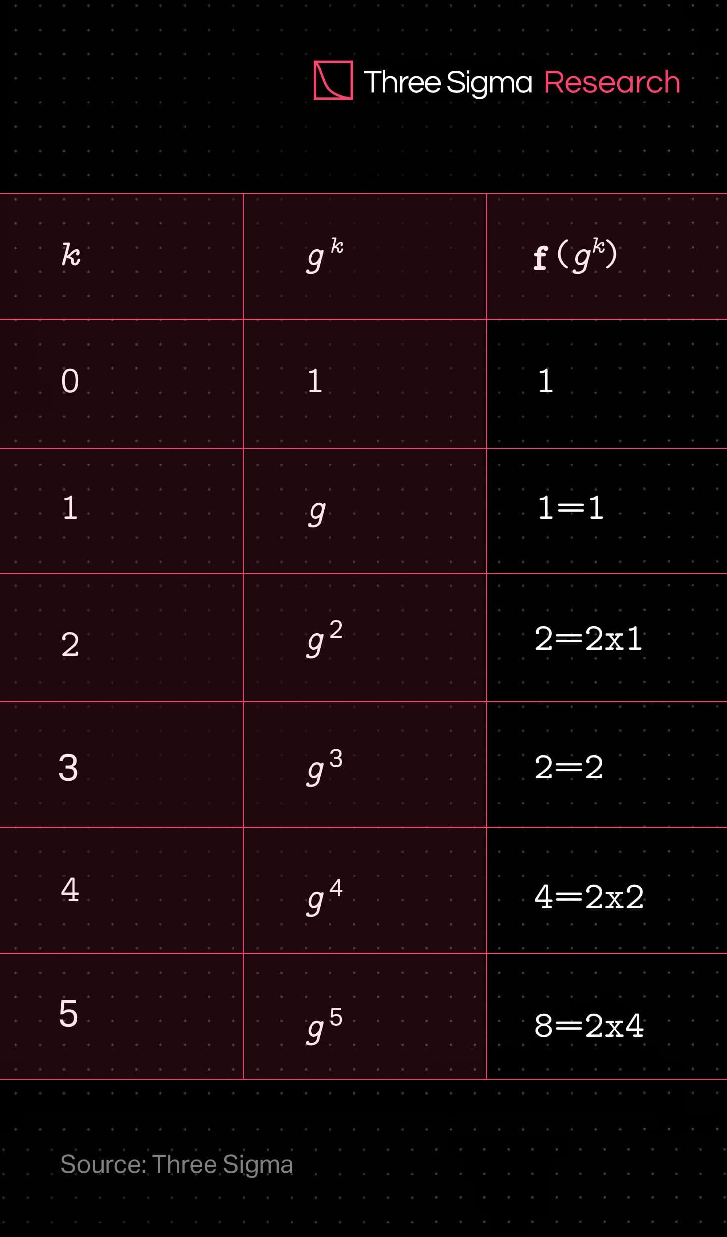
Example: Suppose we have a trace table that is subject to 3 different constraints:

These can be interpreted as:

• in row , the trace value must be ,
• in rows and , the trace value must equal the previous one, and
• in rows , and , the trace value is double the previous one.

A valid trace for this set of constraints would be:

‎

Preprocessed AIR (PAIR)

Preprocessed AIR is an arithmetization procedure that combines into a single constraint multiple disjoint constraints, i.e. those that are not enforced simultaneously. This is achieved by appending an extra column of data to the trace table (hence preprocessed), that will act as a selector for the constraints.

It is possible to generalize the idea of the binary selector in the post by Aztec in order to combine multiple constraints. Choose as the indexing set of the disjoint AIR constraints to be combined into a single “larger” constraint. The generalized combined constraint joins disjoint AIR constraints, for which if where . In this case, the selector function will take values in the set such that it selects just one of the possible for activation, namely

The new column will be interpreted as the evaluation of the selector function on the trace domain , as follows.

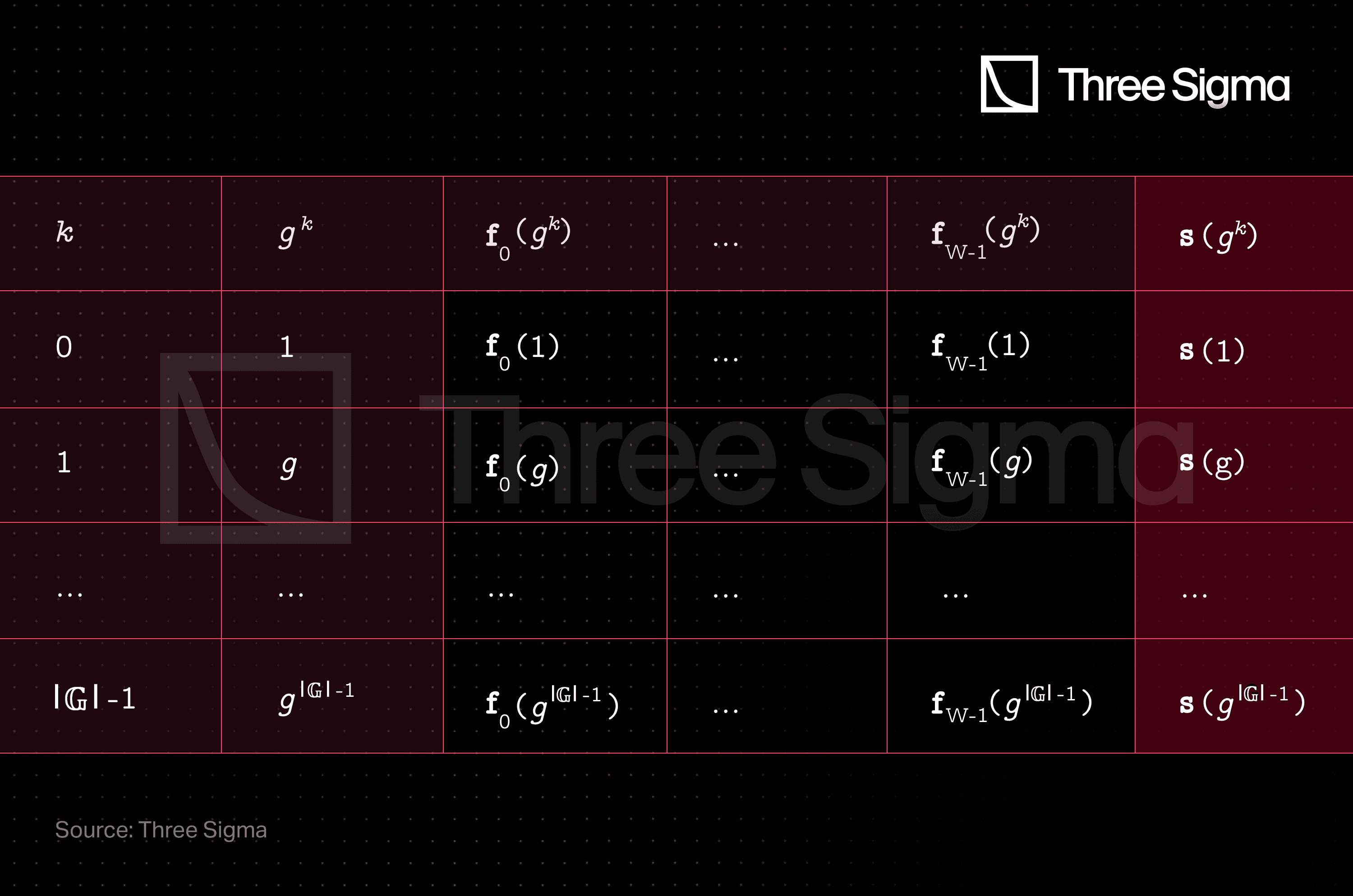
Recall that, in AIR, the constraints indexed by would be statements like

We want to combine all these constraints into a single statement like

To do so, we can simply define the new polynomial as a combination of all the with the use of the selector function , as

where are the optional degree-adjusting random polynomials, and is the vanishing polynomial of the set (if you don’t remember what this is, check Part I). In practice, the selector function will be constructed as the interpolating polynomial of the selector column, to minimize its degree while fulfilling its job.

By inspection, we can see that the function has the following property:

Therefore, in , the function selects just one of the possible for activation, as intended.

Sounds complicated? Let us see how we can apply this formulation.

📝

Continuation of the Previous Example: Recalling the row-wise placement of the constraints, appending the corresponding selector column will result in the following preprocessed trace table:

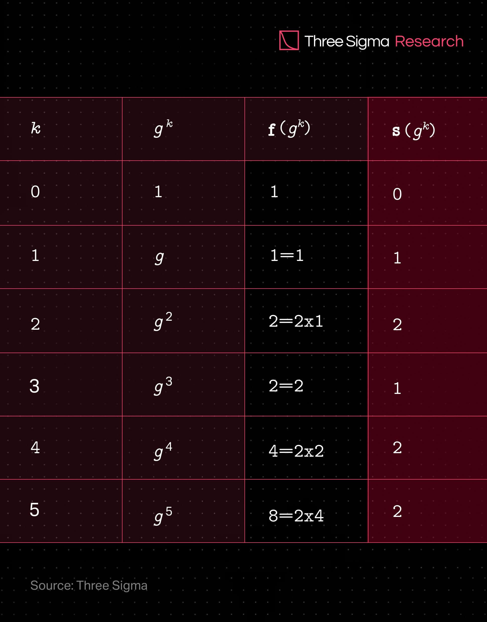
By direct application of equation , the combined constraint polynomial becomes:

You can easily check that:

thus enforcing the intended constraints at their proper enforcement domains.

As explained in the paper, this combined polynomial has a tight degree bound of:

Recall that these are the multivariate AIR polynomials and that their degrees measure how many times the trace function appears in a multiplication, in said constraint. For example, corresponds to , and would have .

‎

Algebraic placement and routing in PAIR

Next, we’ll perform the APR as we would to an AIR constraint, but noticing that the new enforcement domain is simply the disjoint union of all the individual , which we called . As such, if the function has a root for every element of (an honest prover situation), then

defines a new polynomial suitable for low-degree proximity testing. Hence, we can derive the degree bound for this polynomial in an honest prover situation as

which utilizes the tightest degree upper bound known by the verifier. Concerning completeness, this constraint holds if the original computational integrity statement is valid. Pertaining to soundness, if random algebraic linking is not utilized, the reverse implication is also true; otherwise, the equivalence is “merely” very likely.

‎

Wrapping Up

With this post you are now able to convert the enforcement of disjoint AIR constraints into a single, larger constraint, resorting to only one all–encompassing enforcement domain. In the next post we’ll compare how these two distinct methods fare in regard to the degree bounds that they yield for Reed-Solomon proximity testing. You will not want to miss Part III of this series!