Arithmetization in STARKs: Understanding the Foundations
This series is a high-level exploration of the paper Study of Arithmetization Methods for STARKs.
As blockchain transaction volumes increase, scalability and performance optimization are critical concerns. STARKs offer a promising solution, but their security implications and computational requirements must be considered for optimal performance. In this Series, we will be focusing on two arithmetization methods for STARKs, AIR and its variant, PAIR, and their soundness implications for Reed-Solomon proximity testing, RPT—i.e., checking whether functions look like polynomials of low-degree). We will compare these methods regarding degree bounds for RPT.
Part 1 of this series explores the arithmetization of computational integrity statements using AIR. It creates an equivalence between execution trace validity and the specific properties of carefully constructed polynomials. Let’s get to it!
Arithmetization and Algebraic Intermediate Representation (AIR) in STARKs: Background
Arithmetization is a technique that reduces computational problems to algebraic problems using low-degree polynomials over a finite field. In STARKs, arithmetization encompasses three stages: Algebraic Intermediate Representation (AIR), Algebraic Placement and Routing (APR), and Algebraic Linking IOP (ALI). AIR is used to translate computational integrity statements into relations and properties of polynomials. APR transforms AIRs into Reed-Solomon membership problems, and ALI combines these problems into a smaller set of Reed-Solomon proximity problems using public randomness.

Execution Trace in Arithmetization: A Key Component
Before we go any further, we should clarify how we define the execution trace. A program's execution trace records the different states of the program/machine as it runs. These states are separated by clock cycles and given a value that encodes important parameters. The states can be represented either by a collection of state variables or by a single value that combines all of these. Because computational operations are discrete, finite fields are used to assign values to state variables, which also avoids numeric overflow and underflow.
In general, the trace function maps from a finite field to the multidimensional space of state variables . We will represent the evaluation of using a table with columns (the width).
The execution trace is built from the evaluation of on a domain which has some special properties:
- is a subset of with elements (its cardinality, or group order), and
- There exists an element such that .
The execution trace may can be represented with a table like this one:
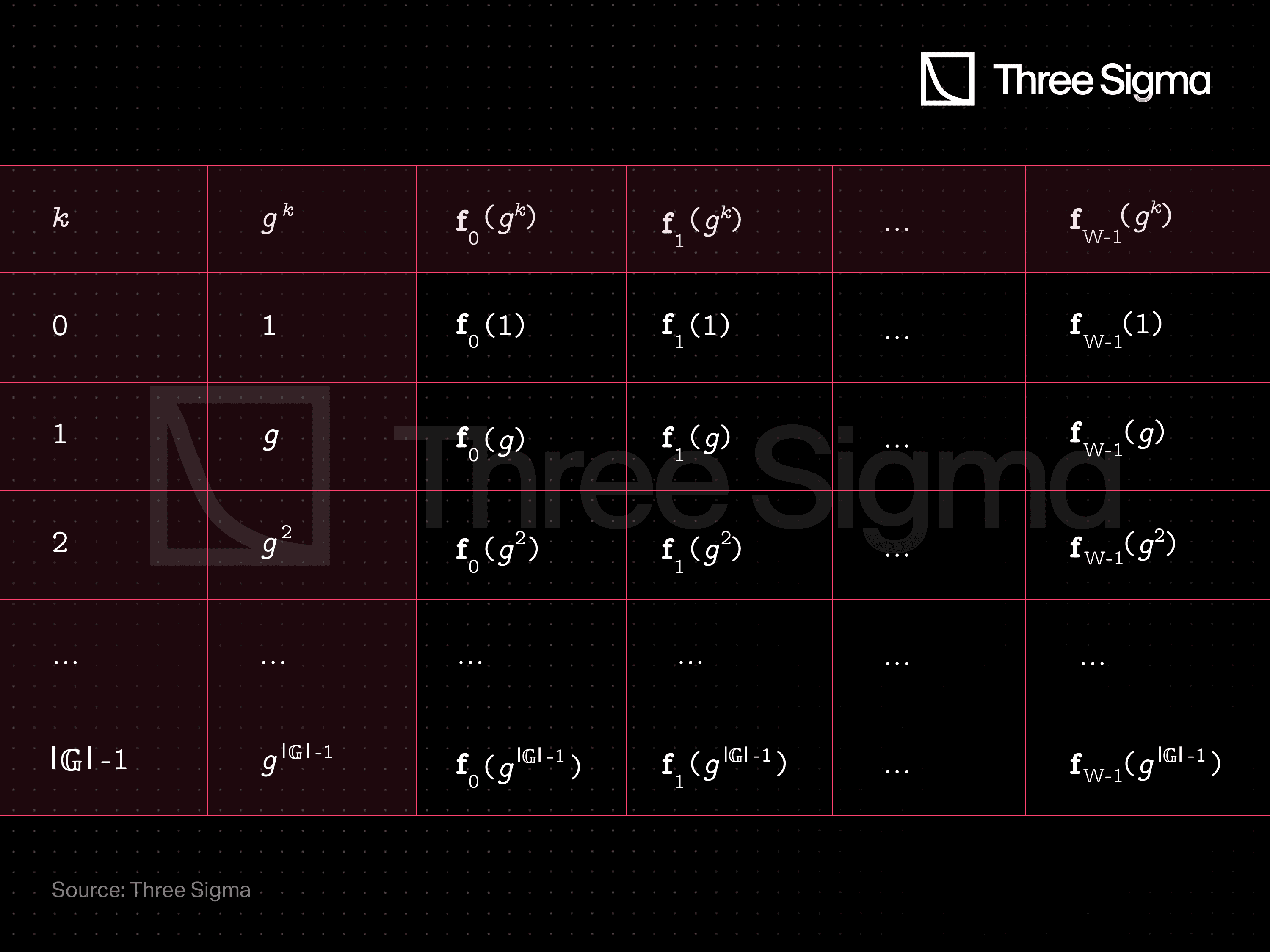
Each row represents the state of the machine in a specific clock cycle, and they are associated to the consecutive powers of . In this context, all columns of the trace can be interpolated into polynomials of degree , by using Lagrange interpolation, for example . As such, the trace function is uniquely defined from the execution trace.
For the purposes of these posts, a polynomial is a finite expression involving addition and multiplication between the variables and scalar values in the field , and that outputs a value in as well.
Algebraic Intermediate Representation (AIR): Defining Computational Integrity
In STARKs, an algebraic intermediate representation is a high-level description of arithmetic constraints for computations. The computational integrity statement is enforced via constraints which are expressed as polynomials composed over the execution trace.
Besides specifying , and , to define an AIR we require a set of constraints. Let be a subset of that indexes the set of constraints. For , the th constraint is a collection of
- the th enforcement domain, , which is a subset of
- the th mask, , which is a list of length , and
- the th multivariate polynomial, , that takes in field elements and outputs a single field element.
These components allow us to rewrite the computational integrity constraints as polynomials!
To make it more simple, we have the multivariate polynomial . We would like the variables to correspond to elements of the trace table, which should be constrained to translate the computational integrity statement. These elements may be specified using the columns and rows of the table. This is the objective of the mask, which is a list like
The elements of the mask are of the type . Here, and are utilized to specify the column and row-offset on the trace table. The main idea is that the we can substitute arguments of with for each of the . Hence we would have the AIR assignment:
Example:
Consider the sum constraint
This should read as ”for rows 0 and 1, the trace elements in column 2 should be equal to the sum of the trace elements in columns 0 and 1 of the previous rows”. We would define the constraint elements as
such that enforces the sum constraint at , i.e. the first two rows.
Without getting to much into the details of how the mask itself works, we will simplify this construction as
This means that the computational integrity statement is valid if these functions evaluate to zero on some specified points. Hence, computational integrity was reduced to checking the roots of polynomials! You can see more details in Section 3 of the paper.
Algebraic Placement and Routing (APR) in Arithmetization
In APR, the AIR instance and witness are directly mapped to a set of Reed-Solomon proximity problems (whether the functions look like polynomials of low-degree). To build this new framework, we’ll define as the vanishing polynomial of a set , yielding
Observe that it evaluates to zero at all the points of the associated set: for all .
If the function has a root for every element of (an honest prover situation), then the expression
defines a polynomial of degree
yielding as a tight upper bound for the degree of , acknowledged by both the verifier and the prover. These new polynomials generate useful Reed-Solomon membership problems: to be or not to be of low-degree.
- In the case of an honest prover, the numerator will have factors that cancel the vanishing polynomial in the denominator, since for any , effectively resulting in a with degree at most.
- For a dishonest prover, at least one constraint will not hold in its enforcement domain, and the denominator will not be cancelled, resulting in a rational function that is not a polynomial of degree at most .
Thus, APR yields constraints that are equivalent to the corresponding original computational integrity constraints.
Before proceeding, the prover must commit to the low-degree extension of the trace function, . This means that the prover must evaluate this function on a large domain (that was previously agreed upon between the prover and the verifier) and then publicly commit that data to an immutable database (a Merkle-tree should do the job).
Algebraic Linking IOP (ALI): Finalizing Arithmetization
ALI, the final step in arithmetization, reduces the number of Reed-Solomon proximity tests required by constructing the composition polynomial. The basic idea behind ALI is to use public randomness to combine the polynomials into a single low-degree polynomial. This process involves a verifier-prover interaction (the I in ALI), which can be made non-interactive using the Fiat-Shamir transform.
One of the main advantages of ALI is that it limits the prover's ability to influence proximity testing, due to the injection of randomness. By making it computationally unfeasible and probabilistically unlikely for the prover to manipulate the APR polynomials, the ALI polynomial is less likely to lie within a desired outcome for the subsequent proximity testing. In other words, when the input instance is unsatisfiable, the ALI generates RPT problem instances that are significantly distinct from low-degree polynomials (see Section 1.4 of the DEEP-FRI paper).
After the prover has committed to the low degree extension of the trace, they can create the composition polynomial by combining the individual , which under an honest prover situation have , with . In its general form, the verifier provides random polynomials over the algebraic extension field (larger fields promote security) such that the composition polynomial becomes
where are degree-adjustment polynomials that ensure that all of the constraints are treated equally in the low-degree analysis, and inject randomness into the process of combining the constraints, promoting security. Particularly, one regulates the degree of by choosing such that , adjusting the degree-bound of the corresponding constraint as
If is a polynomial of degree lower than , the corresponding APR polynomial, , has degree at most , as intended.
- In an honest prover situation, the degree of the composition polynomial is bounded as .
- In a dishonest prover situation, as a consequence of the APR reduction, at least one of the will not respect the degree bound. Hence, it is very unlikely that respects this degree bound either, as the sum of random high degree polynomials rarely results in a low-degree polynomial.
This should be tested by the subsequent RPT (again, FRI is perfect for the job).
Wrapping Up: The Role of Arithmetization in STARKs
You have now been introduced to the main steps of constraint arithmetization for STARKs! In the next post we’ll dive deeper into the details and explore an alternative method to coordinate the enforcement of constraints: PAIR - Preprocessed AIR.

Researcher
João holds a Master's degree in aerospace engineering from Instituto Superior Técnico. He is always eager to learn and is particularly interested in the analytical aspects of various subjects. João joined the research department at Three Sigma as he considers it to be an interesting challenge that will require him to diversify his skill set. In his free time, he enjoys mountain biking and playing tennis.
Researcher
Tiago has a Bachelor's and Master's degree in aerospace engineering from Instituto Superior Técnico and profound experience in nonlinear structural dynamics from Technical University of Munich. His interests in mathematics, cryptography, and computational algorithms make him well-suited for research in algorithms for cryptographic proofs. He focuses on understanding, improving, and building Zero-Knowledge primitives such as STARKs and SNARKs, in Three Sigma’s research department, offering valuable expertise and unique perspectives on the future of crypto technology.